Skip navigation
2014

The columnar storage is good, especially when there are lots of tabular fields (this is quite common). In querying, the data to traverse is far less than that on the row storage. Less data to traverse brings less I/O workloads and higher query speed. However, the Hadoop application consumes most time on the hard disk I/O without columnar storage.

Both Hive and Impala support columnar storage, but columnar storage only available with the basic SQL interface. As for some more complex data computing, it seems quite difficult for the MapReduce framework to do columnar storage.

The sample data is a big data file sales.txt on the HDFS. This file has twenty fields, 100 million data entries, and the file size is 14G. Let’s take the GROUP computing for example to demonstrate the whole procedure. Concretely speaking, it is to summarize the total sales for everyone by the sales person. The algorithm involves two fields, empID and amount.

Firstly, compare it with the classic code for Grouping and Summarizing on Columnar Storage:

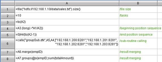
Code for summary machine:

columnar_storage.png

Code for node machine:

columnar_storage_2.png

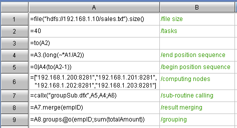
The above columnar storage algorithm follows such train of thought: Scheduling a large task into forty smaller tasks according to the file bytes; distribute them to the node machine for the initial summarization; and then further secondary summarize on the summary machine. This train of thoughts is similar to that for MapReduce. The difference is that this columnar storage thinking pattern is simple and intuitive because the task scale could be customized, and most people can understand it easily.

As can be seen, the row storage is to store all fields in the file in the form of fields. Therefore, no matter there are two or twenty fields, we still have to traverse all data – the file of 14 G. However, the columnar storage is not like this. The data of each field are stored as a file. If only two fields are stored in the query, then you only need to retrieve the corresponding file of these two fields, i.e. 1.4 G. Please note that the 1.4 G is an average value. The total volume of the data of the two fields is slightly higher than 1.4 G.

As mentioned above, to implement the columnar storage, we must decompose the file field by field first, by using f.cursor() to retrieve first and then f.export() to export. The detailed procedure about columnar storage will be explained at the end of this article.

Code for Grouping and summarizing once Columnar Storage is adopted:

Code for summary machine:

columnar_storage_3.jpg

Code for node machine:

columnar_storage_4.png

As can be seen, the greatest change is the code for node machine. The A3 cell uses the [file list]. Use the cursor() to merge a group of field files to generate a cursor of 2 dimension table. The remaining codes for grouping and summarizing are just the same as before.

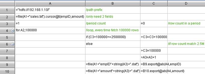
Another change is about the task-scheduling. In fact, great trouble can be caused in this stage. As we know, in the row storage, the task-scheduling can be performed based on the number of byes. For example, a 14 G file can be divided into 40 segments evenly, and each segment will be assigned to a node machine as a task. But this method does not work in the columnar storage because of the record misalignment, and the result can be always wrong. The right method is to divide evenly by the number of records (Any suggestions on dividing it evenly, please leave a comment. Thanks.). 100 million entries can be allocated to 40 segments, and each segment will hold 2’500’000 entries.

For example, the empID column will be ultimately divided into 40 smaller files: empID1. dat”,”empID2. dat”……”empID40. dat”. Then, the algorithm codes are shown below:

columnar_storage_5.jpg

In order to prevent the memory overflow, the above algorithm will retrieve 100’000 entries from cursor, and append to the file. By doing this, a new file will be created with every 2’500’000 entries of data. In which, A3 is the file count, C3 is used to monitor if the data entries in the current files reaches 2.5 M.

The data-scheduling is surprisingly troublesome, but the columnar computing after splitting is quite simple.

Web: http://www.raqsoft.com/

raqsoft

6 Data Computing Tools

Posted by raqsoft Jan 23, 2014

Recently, I finished a project which involves using the Excel, R Project, and es-series in combination. An idea occurred to me in the work. Why not put them along with the Matlab, SPSS, and Stata side-by-side to make an introductions and comparisons of Desktop BI tools? At last, this essay comes into being, as you can see below.

Desktop BI refers to the BI tools running on the desktop environment, almost not requiring any server supports. The typical Desktop BI only provides the core BI functions with less requirement on the technical environments. By comparison, such software as Solution BI cannot operate without the support from private server. They are usually the integrated solution or platform system in-built with lots of half-finished components. Besides the core BI functions, Solution BI also provide some non-core functions like the authority management, resources sharing, and collaboration between jobs of various types. Desktop BI is the commonest tool for people doing the data computing and analysis.

Comparison results:

Technical Requirements:              Excel > ES Series> SPSS >Matlab >STATA >R

Numbers of statistical models:   R >STATA >SPSS >Matlab >Excel >ES Series

API capability:           R >Excel > STATA > Matlab >SPSS >ES Series

Complex computing goal:      ES Series  >R >Matlab >Excel >STATA >SPSS

Graphic capability:                  SPSS >R > Matlab  > ES Series  >Stata >Excel

Learning curve:              Excel > SPSS > ES Series >Matlab >STATA >R

Interactive computing:      ES Series  > Excel  >R >Matlab >STATA >SPSS

Price:                         R >Excel >ES Series >Stata >Matlab >SPSS

Note: In the above comparison, the tool on the left has more advantages than those the right.

Excel

Of all BI software, which one occupies the largest market shares, has the largest user base, and experiences the greatest increase in each year? It is neither QlikView / Spotfire, nor SAS / SAP, but Excel. Does it surprise you? BI producers are always running down Excel in an attempt to describe Excel as “inferior BI toy” or even “outdating BI”. But the figures won’t lie, Gartner, many true BI users, and even these producers have to admit that Excel is the most (not just the one of the most) important BI tool.

Excel is an intuitive and flexible Desktop BI tool of low technical threshold. BI is aimed to solve the “Business” problem. Who understand the business best? Needless to say, it is the business experts – the core users of BI software. Most of them do not have strong technical background, so they wish the technical threshold will be as low as possible. It seems Excel lack the computing capability and it is hard for Excel to handle the abstract data structure as the SQL and other script languages do. However, confronting the intuitive data directly, Excel has the advantage of providing a flexible and natural computing method. The business experts can be benefited to turn their business algorithm into computer languages according to their business thoughts. This is great expression ability of BI tools. Although other BI tools are more powerful in computing, they are too difficult for business experts to use in expressing the business algorithms. Therefore, no matter how powerful computing capability these tools have got, the business experts cannot leverage it.

R Project      http://www.r-project.org/

R Project holds the largest market shares of open source BI tools. In the KDNuggets survey 2012 on the “Top Analytics, Data Mining, and Big Data software used”, R won the top one title with 30.7% of votes. It is often used for the statistical analysis, matrix computing, and graphic plotting, mainly in the sector of information biology and partly in the economic measurement, financial analysis, and cultural sciences.

R features the interactive computing environment and the abundant 3rd party library functions. R offers an intuitive way to view and make reference to the results of previous computing. Relying on the agile and elegant syntax, R users can carry forward the data processing step by step, and decompose the complex computing goal into several simple goals easily. Such interactive computing environment is ideal for solving the complex and ambiguous BI problems. R is the open-source software with massive function libraries and rapidly updating algorithms. Its secondary development interface supports various languages for users to integrate the 3rd party library functions easily, so it becomes widely popular with a great many users.

Comparatively, R suffers some drawbacks on UI friendliness and technical requirements, which hinders R from further popularization. RStudio and the alike tools can remedy the weak points of R on UI friendliness. However, it is still a far cry from the business software, and the technical requirement on languages is native and unchangeable. Moreover, many people also complain on the relatively low computing speed and the unsatisfactory accuracy of package from the 3rd party.

Last, thanks to the powerful computing capability and the open source characteristic of R, various big data solutions like Teradata , SAP, Oracle, and IBM all declared their support for R and R thus holds the spotlight.

ES Series      http://www.raqsoft.com

ES Series is the next generation Desktop BI tool of the most promising one in making a breakthrough on the traditional BI. Regarding the spreadsheets sector, es-series provides a more powerful computing capability than Excel, quite suitable for the business personnel without technical background to conduct the complex data computing. It implements the homocell model and the visualization of computing procedure. es-series not only allows for the intelligent formula-pasting to reduce the manual operations dramatically and the free step-by-step computing to implement the free data manipulation, but also provides the all-around set computing ability to solve the complex computing easily. The users of es-series tools can perform the table association operation to implement the computing between multiple tables with none formula required. These advantages are always the bottlenecks for the traditional spreadsheets.

Regarding the data computing scripts, es-series tools have the same complete structural data computing ability as SQL, with much lower technical requirements. es-series tools are the same capable as R in its interactive computing abilities to solve the complex problems, and offer a friendlier interface. The syntax of es-series is more intuitive and easier-to-understand. It is the computing scripts that business personnel can grasp easily. Considering its distinguishing features, es-series is superior to SQL or R on many respects. For example, es-series can reach the complex goal of computing more easily through the step-by-step computing in the cellset; its support for explicit sets allows for the intuitive data manipulation from business perspective, and will ultimately reduce the difficulty and improve the readability; es-series tools enable the object reference to implement the associative access to multi-tables intuitively, and support the sorted set to solve any tough problems related to orders.

However, es-series tools comparatively lack such model algorithm as regression analysis, collaboration, and sharing that Excel provides.

SPSS      http://www-01.ibm.com/software/analytics/spss/

SPSS is reputed for its simplicity and friendliness and occupies the greatest market share. SPSS provides the completely graphical UI for operations and the command options of menu style, so that users can perform the commonest module analysis without any scripting. With regard to the fixed module analysis, SPSS is really good at the ANOVA and Multivariate Statistical Analysis. They even do better than SAS of Solution BI in this aspect.

The overall ability in graphic drawing of SPSS is the best among all Desktop BI software. Although the drawing plotted by R is also quite fine, the interactive plotting procedure of SRSS can overtake R completely. Almost everything in the drawings can be altered. No matter it is the statistic chart design stage or the graphic result stage, users can directly alter the colors and line patterns. They can also add the marking variables in the Scatter Diagram or even change the 2D to 3D, or delete some data, or change the basic type of drawings, for example, change the bar charts to the line charts, and add several auxiliary lines at will. Drawing with SPSS will give you a feeling of acting willfully.

However, SPSS is comparatively rather rigid, and only capable to perform the analysis on fixed model. It is quite hard for SPSS users to perform the computing outside the models. For example, firstly, filter the analysis result by the keyword; then rank by another column; secondly, retrieve the several top rankings; and lastly convert the unit of values in a certain column from US Dollar to the Pound. In this aspect, it is quite natural that the computing scripts of R, esProc, and MATLAB are more powerful. Therefore, SPSS cannot be used for free computing and complex analysis. It is the fool-proof software. In addition, SPSS is quite expensive. STATA is comparatively more cost-effective.

STATA    http://www.stata.com

STATA can be regarded as the tools between SPSS and R, considering the price, interface friendliness, flexibility, and degree of freedom. Almost all SPSS fixed analysis models have the corresponding features in STATA. The differences are that SPSS provides the friendly parameter-inputting interface and result representation interface for analysis, while STATA only provides the command line prompt for input and console text output. In addition, the regression analysis of STATA is more powerful than several other tools, such as OLS. The similar advantageous analyses include the Time series analysis and the Panel Data analysis.

The drawing ability of STATA is also fine and almost at the same level as that of es-series and R, although it is worse than that of SPSS.

I disagree to the opinion held by some people that STATA is the commercialized R. Although the expansibility of STATA is greater than that of SPSS, and the 3rd party vendors can update the algorithm timely, it is still far worse than that of R. In addition, R, es-series, and MATLAB are the most typical computing scripts, which allow for the free analysis in a way similar to programming. By comparison, STATA is a bit rigid and awkward. We can reach this conclusion:

R can provide all features of STATA, while STATA may not have some features of R. SPSS cannot give the desired features for it doesn’t have, STATA can give them in a very awkward and rigid way, R can give them normally, while esProc can give them easily.

MATLAB  http:// www.mathworks.com/products/matlab/

MATLAB is a computing language and interactive environment for numerical calculation, algorithm development, and data analysis, enabling users to create the user interface by plotting the graphic for themselves. Matlab is widely applied in the industrial automation system design and analysis, as well as the sectors of graphic processing, signal processing, communications, finance-modeling & analysis.

At a first glance, it appears that Matlab and R shares many similarities in the UI style, syntax structure, graphic capability, and other aspect. Their differences are great. Matlab is the shortened form of Matrix Laboratory. As the name implies, it is the best at the matrix computation. Matlab can provide more mathematical functions than R. In addition, it can provide many functions based on in-depth study on the specific industries or majors, for example, industrial data analysis, financial model setup, and neural network toolbox. Matlab can do more professionally in these areas than R. Its graphical operation capability is greater than that of R but worse than that of SPSS.

Comparatively, R has stronger language expressing ability and more powerful statistic functions than Matlab. In other words, R is simpler and more flexible to convert the algorithms on paper to the languages that computers could understand. In addition, the statistical module of Matlab is neither complete nor updated.

As to the price of MATLAB, its price is between SPSS and STATA, which is “a little expensive”.

Conventionally, we shall say that each of these tools has its strong point and let’s use them in combination. But according to my years of experiences, I would like to offer an personal advice that the tool capable of expressing your thoughts freely is the tool best for you.

Web: http://www.raqsoft.com/

Hadoop is an outstanding parallel computing system whose default parallel computing mode is MapReduce. However, such parallel computing is not specially designed for parallel data computing. Plus, it is not an agile parallel computing program language, the coding efficiency for data computing is relatively low, and this parallel computing is even more difficult to compose the universal algorithm.


Regarding the agile program language and parallel computing, esProc and MapReduce are very similar in function.


Here is an example illustrating how to develop parallel computing in Hadoop with an agile program language. Take the common Group algorithm in MapReduce for example: According to the order data on HDFS, sum up the sales amount of sales person, and seek the top N salesman. In the example code of agile program language, the big data file fileName, fields-to-group groupField, fileds-to-summarizing sumField, syntax-for-summarizing method, and the top-N-list topN are all parameters. In esProc, the corresponding agile program language codes are shown below:


Agile program language code for summary machine:

Agile program language code for node machine:


How to perform the parallel data computing over big data? The most intuitive idea occurs to you would be: Decompose a task into several parallel segments to conduct parallel computing; distribute them to the unit machine to summarize initially; and then further summarize the summary machine for the second time.


From the above codes, we can see that esProc has parallel data computing into two categories: The respective codes for summary machine and node machine. The summary machine is responsible for task scheduling, distributing the task to every parallel computing node in the form of parameter to conduct parallel computing, and ultimately consolidating and summarizing the parallel computing results from parallel computing node machines. The node machines are used to get a segment of the whole data piece as specified by parameters, and then group and summarize the data of this segment.


Then, let’s discuss the above-mentioned parallel data computingcodes in details.

Variable definition in parallel computing


As can be seen from the above parallel computing codes, esProc is the codes written in the cells. Each cell is represented with a unique combination of row ID and column ID. The variable is the cell name requiring no definition, for example, in the summary machine code:

n  A2: =40

n  A6: = ["192. 168. 1. 200: 8281","192. 168. 1. 201: 8281","192. 168. 1. 202: 8281","192. 168. 1. 203: 8281"]

A2 and A6 are just two variables representing the number of parallel computing tasks and the list of node machines respectively. The other agile program language codes can reference the variables with the cell name directly. For example, the A3, A4, and A5 all reference A2, and A7 references A6.


Since the variable is itself the cell name, the reference between cells is intuitive and convenient. Obviously, this parallel computing method allows for decomposing a great goal into several simple parallel computing steps, and achieving the ultimate goal by invoking progressively between steps. In the above codes: A8 makes references to A7, A9 references the A8, and A9 references A10. Each step is aimed to solve a small problem in parallel computing. Step by step, the parallel computing goal of this example is ultimately solved.


External parameter in parallel computing


In esProc, a parameter can be used as the normal parameter or macro. For example, in the agile program language code of summary machine, the fileName, groupField, sumField, and method are all external parameters:

n  A1: =file(fileName). size()

n  A7: =callx(“groupSub. dfx”,A5,A4,fileName,groupField,sumField,method;A6)

         They respectively have the below meanings:

n  filename, the name of big data file, for example, " hdfs: //192. 168. 1. 10/sales. txt"

n  groupField, fields to group, for example: empID

n  sumField, fields to summarize, for example: amount

n  parallel computing method, method for summarizing, for example: sum, min, max, and etc.

If enclosing parameter with ${}, then this enclosed parameter can be used as macro, for example, the piece of agile program language code from summary machine

n  A8: =A7. merge(${gruopField})   

n  A9: =A8. groups@o(${gruopField};${method}(Amount): sumAmount)

In this case, the macro will be interpreted as code by esProc to execute, instead of the normal parameters. The translated parallel computing codes can be:

n  A8: =A7. merge(empID)   

n  A9: =A8. groups@o(empID;sum(Amount): sumAmount)


Macro is one of the dynamic agile program languages. Compared with parameters, macro can be used directly in data computing as codes in a much more flexible way, and reused very easily.


Two-dimensional table in A10

Why A10 deserves special discussion? It is because A10 is a two-dimensional table. This type of tables is frequently used in our parallel data computing. There are two columns, representing the character string type and float type respectively. Its structure is like this:

         empID

sumAmount

C010010

456734. 12

C010211

443123. 15

C120038

421348. 41


In this parallel computing solution, the application of two-dimensional table itself indicates that esProc supports the dynamic data type. In other words, we can organize various types of data to one variable, not having to make any extra effort to specify it. The dynamic data type not only saves the effort of defining the data type, but is also convenient for its strong ability in expressing. In using the above two-dimensional table, you may find that using the dynamic data type for big data parallel computing would be more convenient.


Besides the two-dimensional table, the dynamic data type can also be array, for example, A3: =to(A2), A3 is an array whose value is [1,2,3…. . 40]. Needless to say, the simple values are more acceptable. I’ve verified the data of date, string, and integer types.


The dynamic data type must support the nested data structure. For example, the first member of array is a member, the second member is an array, and the third member is a two-dimensional table. This makes the dynamic data type ever more flexible.


Parallel computing functions for big data

In esProc, there are many functions that are aimed for the big data parallel computing, for example, the A3 in the above-mentioned codes: =to(A2), then it generates an array [1,2,3…. . 40].


Regarding this array, you can directly compute over each of its members without the loop statements, for example, A4: =A3. (long(~*A1/A2)). In this formula, the current member of A3 (represented with “~”) will be multiplied with A1, and then divided by A2. Suppose A1=20000000, then the computing result of A4 would be like this: [50000, 100000, 1500000, 2000000… 20000000]


The official name of such function is loop function, which is designed to make the agile program language more agile by reducing the loop statements.


The loop functions can be used to handle whatsoever big data parallel computing; even the two-dimensional tables from the database are also acceptable. For example, A8, A9, A10 - they are loop functions acting on the two dimensional table:

n  A8: =A7. merge(${gruopField})    

n  A9: =A8. groups@o(${gruopField};${method}(Amount): sumAmount)

n  A10: =A9. sort(sumAmount: -1). select(#<=10)


Parameters in the loop function

Check out the codes in A10: =A9. sort(sumAmount: -1). select(#<=10)


sort(sumAmount: -1) indicates to sort in reverse order by the sumAmount field of the two-dimensional table of A9. select(#<=10) indicates to filter the previous result of sorting, and filter out the records whose serial numbers (represented with #) are not greater than 10.


The parameters of these two parallel computing functions are not the fixed parameter value but parallel computing method. They can be formulas or functions. The usage of such parallel computing parameter is the parameter formula.


As can be seen here, the parameter formula is also more agile syntax program language. It makes the usage of parameters more flexible. The function calling is more convenient, and the workload of coding can be greatly reduced because of its parallel computing mechanism.


From the above example, we can see that esProc can be used to write Hadoop with an agile program language with parallel computing. By doing so, the code maintenance cost is greatly reduced, and the code reuse and data migration would be ever more convenient and better performance with parallel computing mechanism.


Personal blog: http://datakeyword.blogspot.com/

Web: http://www.raqsoft.com/
The MapReduce of Hadoop is a widely-used parallel computing framework. However, its code reuse mechanism is inconvenient, and it is quite cumbersome to pass parameters. Far different from our usual experience of calling the library function easily, I found both the coder and the caller must bear a sizable amount of precautions in mind when writing even a short pieces of program for calling by others.


However, we finally find that esProc could easily realize code reuse in hadoop.   Still a simple and understandable example of grouping and summarizing, let’s check out a solution with not so great reusability. Suppose we need to group the big data of order (sales.txt) on HDFS by salesman (empID), and seek the corresponding sales amount of each Salesman. esProc codes are:

Code for summary machine:

hadoop_code_reuse_1.jpg

Code for node machine:

hadoop_code_reuse_2.png 


esProc classifies the distributed computing into two categories: The respective codes for summary machine and node machine. The summary machine is responsible for task scheduling, distributing the task to every task in the form of parameter, and finally integrating and summarizing the computing results from node machines. The node machines are used to get a segment of the whole data piece as specified by parameters, and then group and summarize the data of this segment.


As can be seen, esProc code is intuitive and straightforward, just like the natural and common thinking patterns. The summary machine distributes a task into several segments; distributes them to the unit machine to summarize initially; and then further summarizes the summary machine for the second time. Another thing to note is the esProc grouping and summarizing function “groups”, which is used to perform the grouping action over the two-dimensional table A1 by empID and sum up the values of amount fields. The result will be renamed to the understandable totalAmount. This whole procedure of grouping and summarizing is quite concise and intuitive: A1.groups(empID;sum(amount): totalAmount)


In addition, the groups function can be applied to not only the small 2D table, but also the 2D table that is too great to be held in the memory. For example, the cursor mode is adopted for the above codes.


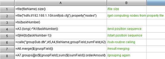
But there are some obvious defects in the above example: The reusability of code is not great. In the steps followed, we will rewrite the above example to a universal algorithm independent of any concrete business. It will be rewritten to control the code flow with parameters, so as to summarize whatsoever data file. In which, the task granularity can be scheduled into arbitrary number of segments, and the computing nodes can be specified at will. Then, the revised codes are shown below:


Code for summary machine. There are altogether 4 parameters defined here: fileName: Big data file to analyze; taskNumber: Number of tasks to distribute; groupField: Fields to group; sumField: Fields to summarize. In addition, the node machine is obtained via reading the profiles.

hadoop_code_reuse_3.jpg 


Code for node machine. In the revised codes, 4 variables are used to receive the parameter from summary machine. Besides the file starting and ending positions (start and end) from the first example, there are two newly-added fields. They are groupField: Fields to group; and sumField: Fields to summarize.

hadoop_code_reuse_4.png


In esProc, it is much easier to pass and use parameter because users can implement the common grouping and summarizing with the least modification workload, and reuse the codes easily.


In Hadoop, the complicated business algorithm is mainly implemented by writing the MapReduce class. By comparison, it is much more inflexible to pass and use parameters in MapReduce. Though it is possible to implement a flexible algorithm independent of the concrete business, it is really cumbersome. Judging the Hadoop codes, the coupling degree of code and business is great. To pass the parameters, a global-variable-like mechanism is required, which is not only inconvenient but also hard to understand. That’s why so many questions about MapReduce parameter-passing are here and there on many Web pages. Lots of people feel confused about developing universal algorithms with MapReduce.


In addition, the default separator in the above codes is the comma. It is obvious that users only need to add a variable in a similar way to customize it to any more commonly-used symbol. With it, they can also implement the common action of data filtering and then grouping and summarizing easily. Please note the usage of parameter groupField. It is used as the character parameter in the cell A6, but the macro in A8. In other words, ${gruopField} can be resolved as the formula itself, instead of any parameter in the formula alone. This is the work of dynamic language. Therefore, esProc can realize the completely flexible code, for example, using the parameter to control the summary algorithm to perform sum up or just count, seek the average value or maximum.


“Macro” is a simple special case of dynamic language. esProc supports a more flexible and complete dynamic language system.


  As you may find from the above example, esProc can implement Hadoop code reuse easily, and basically achieve the goal of “Write once, run anywhere!”. Needless to say, the development efficiency can be boosted dramatically.